

트랜스포머 모델은 자연어 처리에서 가장 기본이 되는 모델로 구글이 발표한 논문인 "Attention is all you need"에서 처음으로 나온 모델이다. 기존의 seq2seq의 구조인 인코더-디코더를 따르면서도, 어텐션(Attention)만으로 구현한 모델이다. 이 모델은 RNN을 사용하지 않고, 인코더-디코더 구조를 설계하였음에도 번역 성능에서 RNN보다 우수한 성능을 보여주었다.
Input Embedding

트랜스포머 아키텍처는 위의 그림과 같이 생겼다. 먼저 첫 단계인 빨간 박스의 Input Embedding부터 알아보자. 먼저 입력으로 들어오는 단어들을 임베딩 벡터로 바꿔줘야한다.

예를 들어 단어가 어휘 사전에서 1,918번째에 위치한다면 1,918로 변환된다.(원-핫 인코딩은 단어 집합 크기와 동일한 차원을 가져야해서 고차원의 벡터로 변환되면 GPU가 연산하는데 불필요한 메모리 사용하기 때문에 불필요한 메모리 과다 소비를 방지하기 위해서 사용하지 않는다.)
그 후 단어 개수만큼 행을 가지는 임베딩 행렬(룩업테이블)에서 인덱스 1,918번에 위치한 행을 단어 great의 임베딩 벡터(밀집 벡터)로 그대로 사용한다.
※ 임베딩 행렬은 [어휘 사전의 크기, 임베딩 차원] 의 크기를 갖는다.
※ 룩업 테이블의 값들은 초기에 랜덤값으로 설정된다.
※ 임베딩 행렬은 일반적으로 모델의 학습 과정에서 최적화되는 파라미터 중 하나이다
※ 학습 한다는 것은 문맥상 유사도가 높다면 임베딩 벡터값을 점점 가깝게 변경 한다는것
Positional Encoding

다음은 Positional Encoding(위치 인코딩)이다.위치 인코딩이 필요한 이유는 input에 입력되는 값을 순서대로 처리되는 RNN이나 LSTM과 다르게 연산을 빠르게 처리하기 위해 input에 한꺼번에 병렬로 값을 처리하는 트랜스포머는 단어의 위치를 알 수 없게 된다.(어텐션은 동시에 처리하기 때문에) 그래서 위치 인코딩 레이어를 사용한다.

예를 들어 트랜스포머에서는 “dog bites man”와 “man bites dog”는 뜻이 다르지만 같은것으로 인식한다. 왜냐하면 각각의 토큰들은 모두와 이어져있기 때문에 추가적인 위치 정보없이 토큰의 임베딩 정보만으로 두 문장의 차이를 구분할 수 없다. 그래서 같은 단어 임베딩이라 할지라도, 고유한 위치정보를 같이 준다면, 개가 사람을 물었는지 사람이 개를 물었는지 위치 인코딩을 해주는것이다.

위치 인코딩은 위와 같은 수식으로 단어의 위치를 인코딩한다.

이렇게 계산된 위치 임베딩과 입력 임베딩을 각 행에 맞게 더해주기만 하면 입력+위치 임베딩 벡터를 구하게 된것이다.
이제 임베딩 벡터에 포지셔널 인코딩의 값을 더하였으니 같은 단어라도 문장 내의 위치에 따라 트랜스포머의 입력으로 들어가는 임베딩 벡터의 값이 달라진다!
Multi-Head Attention

멀티헤드 어텐션은 어텐션을 한번에 처리하는것 아닌 여러 개로 분할하여 즉 멀티헤드로 셀프 어텐션을 다양한 관점에서 하게 만들어 더 강력한 모델을 만들기 위함이다.

셀프어텐션은 입력 문장 내의 단어들끼리 유사도를 구하는것이다. 이 유사도를 통해 이제 기계는 “철수는 물건을 건내주지 않았다. 왜냐하면 그것은 너무 무겁기 때문이다.” 라는 문장에서 ‘그것’ 이라는것이 ‘물건‘을 뜻하는것을 알게 되는것이다.
셀프 어텐션을 통해 기계는 문맥을 더 잘 이해할 수 있게 되고 복잡한 질문에서도 중요한 부분을 파악하고 올바른 출력을 할 수 있게된다.
[Attention의 구성요소]
Query : 정보를 가져올 근거(질문)
Key : 가져올 정보의 고유 식별 값
Value : 실제로 가져올 값

멀티헤드 어텐션의 구조는 위의 그림과 같다. 멀티헤드 어텐션의 입력으로 들어가기 전 Query와 Key를 이용해서 Value 가운데 어떤 값을 어느 정도 가져올지를 계산해서 그 가중치를 뽑아주게된다. 우선 Q, K, V 벡터를 구하기 위해 빨간 박스인 Linear Layer를 거쳐야한다. (기존 벡터로부터 가중치 행렬을 곱해야함) 그 과정을 살펴보겠다.
※ Linear Layer를 거치는 이유는 Query, Key, Value의 차원을 줄여서 병렬 연산에 적합한 구조를 만들기 위해서이다.

왼쪽그림의 빨간박스인 과정처럼 우선 각 단어 벡터들로부터 Qurey벡터, Key벡터, Value벡터를 얻는 작업을 해야한다.

우리가 구했던 입력+위치 인코딩한 행렬을 세 개로 복사한다.

그리고 쿼리, 즉 Q행렬을 구하기 위해서 d*d크기의 가중치 행렬을 만들어준다. 가중치 행렬은 차원*(차원/헤드 개수)의 크기를 갖는데 논문에서는 512차원에 헤드 개수 8개이지만, 여기서는 편의상 6차원에 헤드 개수는 2개라고 가정한다. 그러면 사진의 오른쪽처럼 6*3 크기의 행렬 2개가 나오는것을 확인할 수 있다.
※ 가중치 행렬은 적절한 범위 내에서 랜덤값으로 설정된다.

그리고 입력+위치 인코딩한 행렬과 가중치 행렬과 행렬곱을 해서 Q 행렬을 구한다. 이렇게 행렬 곱셈을 통해 벡터의 차원을 변경하는것을 선형(Linear)변환 이라고 한다.

이렇게 Q행렬을 구한것처럼K,V도 동일하게 적용하여 Q,K,V 행렬을 만들어낸다. 이제 이렇게 구한 Q,K,V 행렬 값을 다중헤드 어텐션 입력값에 넣어준다.

이렇게 Q, K, V 행렬을 얻었다면 다음은 MatMul(행렬곱) 차례이다.

Q와 K의 행렬곱 공식은 다음과 같다. 이 수식을 사용하여 행렬곱을 해준다. K행렬에 Transpose를 해줘야한다는걸 잊지말자

이렇게 Attention Score를 얻게된다. Attention Score란 Query와 Key 행렬의 행렬곱으로 여기서 행렬곱은 행렬 간의 유사도를 의미하기 때문에 Attention Score는 Query와 Key 사이의 유사도 행렬을 나타낸다.
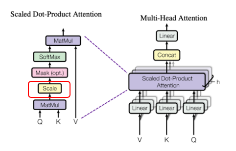
다음은 크기변화(Scale)을 해줘야한다.

앞서 구한 Attention Score에 d(k)에 루트를 씌어준것으로 나눠준다. d(k)는 d(model) / num_heads 라는 식에 따라서 결정되고, 논문에서는 d(k)의 값은 512/8 =64로 √ 64인 8의 값으로 나눠줘야하지만 여기 예제에서는 차원은 6, 헤드수는 2로 설정하였으니 √ 3으로 나눠줘야한다. Scale을 해주는 이유는 내적 유사도의 문제 때문이다. 내적할 두 벡터의 길이가 n일 때, 내적 결과는 n개의 원소별 곱셈 결과를 합한 값이므로 n이 커질수록 값도 커지는 경향이 있다. 즉 n이 늘어나면 덧셈해야 할 값도 늘어나기 때문에 값이 전반적으로 커지는 효과가 있다. 우리는 다음 차례에서 소프트맥스 함수에 입력을 해야하는데 소프트맥스 함수에 입력되는 값이 커지게 되면 역전파 계산에서 그래디언트가 작아져 학습이 잘 안되는 문제가 발생한다.

즉 이미지의 분자값인 어텐션 스코어가 커지면 소프트맥스에서 가중치가 유효한 구간인 정의역 구간을 벗어나서 초록색 상자 부분처럼 경사가 완만해진다. 완만해진다는것은 역전파 과정에서 gradient가 작아진다는 뜻인데 모델의 가중치를 수정하기 위해서 적용시켜야 할 값이 작아지니 모델 수정이 잘 안되고 수정이 잘 안되니 학습이 잘 안되게 되는것이다. 그래서 값이 너무 커지지 않게 만들기 위해서 √(𝑑_𝑘 )로 나눠주는것이다.
※ √(𝑑_𝑘 )는 개수에 비례해서 나눗셈이 이루어지니 개수가 짧으면 짧은 대로 적게 스케일링이 된다.

이렇게 크기변화(Scale) 레이어까지의 값을 구하였다.

마스크 레이어는 인코더에서는 사용하지 않는다.(패스)

그 다음 소프트맥스 레이어이다.

소프트맥스 레이어는 행렬의 값을 확률로 바꿔주는 역할을 한다.

이제 이 행렬은 각각의 단어들이 다른 각각의 단어들과 어떤 관계가 있는지 확률로 보여주는 행렬이다. (각 행의 원소들이 확률처럼 합이 1임)

다음은 MatMul(행렬곱) 차례이다.

Value행렬과 행렬곱을 통해 셀프 어텐션이 가미된, 즉 입력+위치+어텐션 임베딩 행렬을 만든다.

다음은 Concat 레이어이다.

포지션-와이즈 피드 포워드 신경망(Position-wise FFNN) 층은 단일 행렬을 처리하므로 행렬들을 concatenate해준다. 우리가 전에 헤드 개수를 2개라고 가정하여 나온 2개의 행렬을 단순히 이어서 붙여준다고 생각하면 된다.(지금까지 우리는 노란색 행렬 하나의 값만 계산하였지만 또 다른 파란색 행렬도 마찬가지로 같은 계산과정을 거친다.)

다음은 Linear 레이어이다.

단순히 전에 concatenate한 행렬에 가중치 행렬을 곱해주는것이다. 각 헤드의 결과는 서로 다른 패턴(예를 들어 사과라는 단어가 512차원의 임베딩을 가진다면 그 중 64차원은 사과의 색에 대한 정보를 표현하고 다른 64차원은 사과의 맛에 대한 정보를 표현할 것이다.)을 포착하기 때문에 ‘linear’층은 각 헤드에서 결합된 정보를 통합된 하나의 표현으로 만들기 위해 ‘Linear’층을 통해 이러한 정보가 결합되면서 더 강력한 표현을 학습할 수 있게 해주는 것이다.

이렇게 멀티헤드 어텐션을 통해 1개 관점에서 계산할 때보다 더 다양한 측면으로 고려하게 되고, 병렬로 계산하게 되어 속도도 빨라진다.
Add & Norm

다음은 Add & Norm 레이어이다. Add는 잔차 연결(Residual connection)을 의미하고 Norm는 층 정규화(Layer Normalization)를 의미한다. 먼저 Add(잔차 연결)에 대해서 알아보겠다.

결론부터 말하면 Add(잔차 연결)은 다중헤드 아웃풋 행렬과 처음 생성한 입력+위치 임베딩과 더하는 과정이다. 잔차 연결은 ResNet이라고 하는 모델로 구현돼서 유명해진 기법이며 특정한 Layer의 연산결과 f(x)와 연산 이전의 값 x를 더하여 함께 다음 단계의 입력으로 활용하는 기법이다. 좀 더 자세히 알아보자

위의 그림은 일반적인 어떤 Layer를 통과하는 모습이다. 그림을 보면 이전 단계의 출력값에서 얻어진 값 x를 가지고 Layer에 입력하면 나오는, 생성되는 값이 그대로 있을것이다. 그러면 이 값을 가지고 또 그 다음 Layer에 입력하는것이다.

그런데 Residual Connection(잔차 연결)에서는 이전 단계에서의 값을 Layer에 입력하면서 생성된 값에다가 Layer의 입력값으로 사용하기 이전 단계의 값을 다시 더해서 다음 단계에 입력해준다. 이게 어떤효과를 가지냐면 어떤 레이어를 거쳐서 나온 결과를 x라고 가정하고 모델이 학습하고자 하는 정답을 y라고 가정하면 y=wx+b 수식처럼 우리가 현재 단계의 Layer에서 하고자 하는 건 x(i)를 이용해서 어떤 계산을 한 다음에 그 결과가 y가 되기를 바라며 학습을 시키는데 y=wx+b 이 수식에 잔차 연결을 적용하게 되면 wx+b가 현재 Layer에서 나온 생성된 출력값이 되고 여기에 입력값인 x를 또 더 해주니 y = wx+b+x로 수식이 바뀌게 된다. 여기서 x를 좌항으로 이항하면 y – x = wx + b의 형태가 되는데 이 식을 이전의 식과 비교해보면 이전 식 y=wx+b은 w와 b 연산을 통해서 배워야 하는 대상이 y였지만 y – x = wx + b식은 w와b를 통해서 배워야 하는 대상이 y가 아니라, y에서 이전 단계의 출력이자 지금 단계에 들어온 입력인 값인 x를 뺀 값이다. 그렇다는것은 현 단계의 모델이 배워야 할 것은 정답과 이전 단계 사이의 오차인 y-x만 배우면 된다는 뜻이다.
우리는 인공지능 모델에 새로운 레이어(연산)를 추가할 때 여러 개의 레이어를 쌓아서 Output을 만들어낸다. 이 Output과 우리가 배우고자 하는 y의 오차를 최소화시키기 위해서 역전파를 수행한다. 간단한 구현으로 신경망을 순진하게 쌓는다면 훈련 중에 그래디언트 문제가 사라지는 문제를 겪을 것이다. 왜냐하면 역전파는 기본적으로 많은 기울기를 곱하기 때문이다.
우리가 가장 이상적인 학습 방식이라고 한다면 층이 깊어질수록 뒤의 레이어가 앞의 레이어에서 배우지 못한것만 배우도록 하여 오차가 점점 줄어들게 학습시키는것이 가장 이상적일것이다. 실제 모델은 그렇게 작동하지 않는다는 한계가 있다. 왜냐? 각 레이어는 하나의 모델이라고 볼 수 있는데 이전 단계에서 나온 결과는 단순히 고유값을 갖는 어떤 특정한 데이터가 되는것이고 우리가 원하는 Output값 사이의 값을 지금 단계에서 새로 학습하는것이다 보니깐 이상적인 방법처럼 오차 부분만 배우는것이 아니라 이전 단계에서 생성된 결과와 Output 사이의 비선형(복잡한) 관계를 깊어진 층에서 새로 계산해야 하는 문제가 생기게 되는것이다. 그래서 매 단계의 학습이 생각보다 쉽지 않고 복잡한 비선형 관계를 새로 학습하는 것이 되는데 Residual Connection을 적용하게 되면 이전 단계의 결과와 정답 사이의 복잡한 비선형 관계를 새로 학습하는것을 해결해준다. 우리가 배워야 할 대상이 y-x=wx+b 수식에서 y–x가 되니깐, 오차만 배우면 되고 앞 부분의 학습은 앞에 맡기고 뒷부분에서는 나머지 적은 부분만 배우면 되는것이다.
y = wx+b+x 수식은 y = f(x)+x의 구조와 같아 이 구조를 통해 y와 x 이전 레이어의 결과 사이에 추가적인 단계가 없는 직접 연결 (y와+x)이 존재하기 때문에 그래디언트가 f(x)를 거쳐서 가는 루트 외에도 y에서 x로 직접가는 루트가 또 존재해 그래디언트를 크게 전달 할 수 있어서 네트워크를 깊게 만들어도 그래디언트 소실 문제가 해결되는것이다.

그림과 같이 사실 논문에서는 우리가 현재 배우고 있는 인코더 블록이 6개 존재한다. RNN처럼 동일한 값에 미래값을 계속 반복해서 넣는게 아니라 같은 구조에 서로 다른 가중치를 갖고 있는 블록이 6개가 있어서 입력값이 6개를 순차적으로 통과해 Output으로 Context Vector가 만들어지도록 구성되어있는데 앞서 배운 잔차연결의 특성 때문에 잔차 연결을 적용하게 되면 Encoder에서 어텐션 연산을 하고 Feed Forward까지 적용된 인코더를 깊게 쌓아도 학습이 잘 이루어지도록 하는것이다.

이제 Add&Norm에서 Norm 부분 즉, 층 정규화(Layer Normalization)를 알아보자 Normalization이란 대상 값들에서 평균을 빼고, 표준편차로 나누어 평균 0, 표준편차 1의 정규분포상의 값으로 변환하여 나타내는 방식이다.
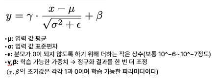
정규화의 수식이다. 각 행의 평균과 표준편차를 구한 후 각 원소에 평균으로 빼준 후 표준편차로 나누어준다.

정규화를 해주는 이유는 모델이 데이터를 입력하기 전에 데이터를 균질한 형태로 바꿔주기 위해서이다. 모델 내부에서 여러 레이어를 거치면서 연산이 거듭되다 보면 값의 분포가 치우치는 현상이 발생한다. 원래 정규분포에서 1,2,3 정도에 수렴하는 분포였는데 값의 분포가 치우치는 형태가 되면 값이 너무 커지게 돼서 그래디언트가 너무 작아지는 Gradient Vanishing 현상이 일어나게 되는 문제가 생기게 되어 학습이 잘 안된다. 그래서 그런 부분들을 해결하기 위해 입력하기 전에 먼저 Normalization 해줘서 전처리를 해주는것 처럼 레이어에 입력되는 데이터를 대상으로 Normalization을 수행하여 값이 과하게 크거나 작은 경우를 재차 조정하여 다음 레이어에 보다 안정적인 입력을 제공하고 또한 레이어의 입력값이 일정한 스케일로 바뀌기 때문에 그래디언트 역시 표준화되어 학습이 잘 되게 하는 효과가 있다. 즉 값이 너무 극단적으로 커지지 않게끔 바꿔주기 위해서 하는 전처리 조치로써 많이 사용하고 이렇게 정규화를 통해 데이터가 들어가게 되면 입력값이 0을 중심으로 한 정규분포의 형태로 고르게 정리되면서 이들을 처리하는 모델 내부의 가중치와 가중치별 그래디언트 역시 안정화되는 효과가 있는것이다.
Feed Forward

트랜스포머 모델에서의 피드 포워드 레이어는 2개의 층으로 이루어진 ReLU()를 활성화 함수로 사용하는 단순한 신경망 구조이다.
Feed Forward 레이어가 존재하는 이유는 뭘까? 지금까지 진행했던 셀프 어텐션에서 여러 가중치 행렬을 곱한것을 기억할것이다. 이런 가중치 행렬을 곱해주는것을 선형 변환이라고 한다.(수학적으로 행렬 곱셈이 덧셈의 보존과 스칼라 곱의 보존 성질을 만족하기 때문) 선형 변환을 한다는것은 선형 함수를 거치는것과 같은데 활성화 함수로 선형 함수를 사용하게 되면 은닉층을 쌓을 수가 없다. 인공 신경망의 능력을 높이기 위해서는 은닉층을 계속해서 추가 해야하는데 만약 인공 신경망에서 입력 신호의 가중치 합을 출력 신호로 변환하는 함수인 활성화 함수를 선형 함수로 사용하게 되면 은닉층을 1회 추가한것과 큰 차이를 줄 수 없기 때문이다.
예를 들어 활성화 함수로 f(x) = Wx라는 선형 함수를 선택하고, 층을 계속 쌓는다고 가정해보자 여기다가 은닉층 두 개를 추가한다고 하면 출력을 포함해서 y(x) = f(f(f(x)))가 된다. 이를 식으로 표현하면 y(x) = W * W * W * x이다. 𝑤^3을 k라고 정의해버리면 다시 y(x) = kx와 같이 표현이 가능하다. 처음 활성화 함수인 f(x) = Wx와 같은 구조이지 않은가? 즉 선형 함수로는 은닉층을 여러분 추가하더라도 1회 추가한 것과 차이를 줄 수 없다. 선형 함수를 사용한 은닉층을 1회 추가한 것과 연속으로 추가한 것이 차이가 없다는 뜻이지, 선형 함수를 사용한 층이 아무 의미가 없다는 뜻은 아니다. 학습 가능한 가중치가 새로 생긴다는 점에서 의미는 있다.
그래서 선형 연산의 문제 해결을 하는 방법으로 Feed Forward Network를 추가함으로써 트랜스포머 모델이 단순한 선형 변환만으로는 캡처할 수 없는 복잡한 관계와 패턴을 학습할 수 있게 되는 것이다. 즉! 셀프 어텐션 내에 비선형 함수가 없는 문제를 어텐션 출력마다 단순하게 비선형 연산을 해 주는 MLP을 더 해 후처리 하는것으로써 해결하는것이다.

Feed-Forward Network의 수식이며 여기서 ReLU함수의 수식은 ReLU(x) = max(0,x)이다

ReLU함수는 음수를 입력하면 0을 출력하고, 양수를 입력하면 입력값을 그대로 반환한다. 렐루 함수는 특정 양수값에 수렴하지 않으므로 깊은 신경망에서 시그모이드 함수보다 훨씬 더 잘 작동한다.

이제 수식에 의해 계산을 해보면 입력과 1층 가중치와 편향을 이용해서 계산을 해주고
(1층 가중치 행렬의 크기는 논문에서는 512*2048)

여기에 ReLU() 활성화 함수를 적용시킨다. (음수 값들은 0이 된다.)

그리고 이것을 다시 2층 가중치와 편향을 이용해 계산해주면, 피드 포워드 레이어의 아웃풋을 계산할 수 있다.
(2층 가중치 행렬의 크기는 논문에서는 2048*512)
Add & Norm

이제 다시 Add & Norm 레이어 차례이다. 아까 배웠던 Add&Norm 레이어를 반복해준다.

먼저 Add 부분으로, 피드 포워드 레이어의 아웃풋과 전에 정규화를 진행했던 아웃풋을 서로 잔차 연결해준다.

다음 Norm 부분으로, Add의 결과에 정규화 과정을 진행해주면 인코더 전체의 아웃풋이 나오게 된다. 이제 이 아웃풋은 같은 구조인 두 번째 인코더 블록으로 입력된다.
참고 자료
[1] https://www.youtube.com/watch?v=p216tTVxues&t=341s
[2] https://www.youtube.com/watch?v=5vOVi3LazdA
[3] https://wikidocs.net/31379
[4] https://wikidocs.net/162098
[5] https://wikidocs.net/60683
[6] https://www.kmooc.kr/view/course/detail/12503?tm=20240804182531
[7]https://www.blossominkyung.com/deeplearning/transformer-mha#0605a67e-d23b-48a5-ad1a-16f32f5c55b3
[8]https://yololife-sy.medium.com/nlp-%ED%8A%B8%EB%9E%9C%EC%8A%A4%ED%8F%AC%EB%A8%B8-multi-head-attention-2-c51a2a1ecf0d